コンテンツにスキップ

Python integration

Python is a rapidly glowing ecosystem for data analysis and visualization in seismology. Followings are some tips & tricks for those who would like to handle the input/output of the OpenSWPC in python. The following example uses

  • ObsPy
  • numpy
  • xarray
  • PyGMT

under the Jupyter Notebook environment.

Input parameter files

A python module OpenSWPC/src/tools/swpc.py contains several utility functions to handle input parameter to the OpenSWPC. To use it, first add this directory to the module path:

1
2
import sys
sys.path.append('/path/to/OpenSWPC/src/tools/')

Then, the module can be loaded as follows:

1
import swpc

A function prm_new() create the default parameter set. These parameters are equivalent to that defined in example/input.inf.

1
prm0 = swpc.prm_new()

Parameter data are stored in a simple dictionary as shown below.

1
print(prm0)
1
{'title': 'swpc', 'odir': './out', 'ntdec_r': 50, 'strict_mode': False, 'nproc_x': 2, 'nproc_y': 2, 'nx': 384, 'ny': 384, 'nz': 384, 'nt': 1000, 'dx': 0.5, 'dy': 0.5, 'dz': 0.5, 'dt': 0.02, 'vcut': 1.5, 'xbeg': -96.0, 'ybeg': -96.0, 'zbeg': -10.0, 'tbeg': 0.0, 'clon': 139.7604, 'clat': 35.7182, 'phi': 0.0, 'fq_min': 0.02, 'fq_max': 2.0, 'fq_ref': 1.0, 'snp_format': 'netcdf', 'xy_ps%sw': False, 'xz_ps%sw': True, 'yz_ps%sw': False, 'fs_ps%sw': False, 'ob_ps%sw': True, 'xy_v%sw': False, 'xz_v%sw': True, 'yz_v%sw': False, 'fs_v%sw': False, 'ob_v%sw': True, 'xy_u%sw': False, 'xz_u%sw': True, 'yz_u%sw': False, 'fs_u%sw': False, 'ob_u%sw': True, 'z0_xy': 7.0, 'x0_yz': 0.0, 'y0_xz': 0.0, 'ntdec_s': 5, 'idec': 2, 'jdec': 2, 'kdec': 2, 'sw_wav_v': True, 'sw_wav_u': False, 'sw_wav_stress': False, 'sw_wav_strain': False, 'ntdec_w': 5, 'ntdec_w_prg': 0, 'st_format': 'xy', 'fn_stloc': './example/stloc.xy', 'wav_format': 'sac', 'stf_format': 'xym0ij', 'stftype': 'kupper', 'fn_stf': './example/source.dat', 'sdep_fit': 'asis', 'bf_mode': False, 'pw_mode': False, 'pw_ztop': 100.0, 'pw_zlen': 30.0, 'pw_ps': 'p', 'pw_strike': 0.0, 'pw_dip': 0.0, 'pw_rake': 0.0, 'abc_type': 'pml', 'na': 20, 'stabilize_pml': False, 'fullspace_mode': False, 'vmodel_type': 'lhm', 'is_ocean': True, 'topo_flatten': False, 'munk_profile': True, 'earth_flattening': False, 'vp0': 5.0, 'vs0': 3.0, 'rho0': 2.7, 'qp0': 200, 'qs0': 200, 'topo0': 0, 'dir_grd': 'dataset/vmodel/ejivsm/', 'fn_grdlst': './example/grd.lst', 'node_grd': 0, 'fn_lhm': 'example/lhm.dat', 'dir_rmed': './in/', 'fn_grdlst_rmed': './example/grd.lst', 'rhomin': 1.0, 'fn_rmed0': 'dummy.ns', 'green_mode': False, 'green_stnm': 'st01', 'green_cmp': 'z', 'green_trise': 1.0, 'green_bforce': False, 'green_maxdist': 550.0, 'green_fmt': 'llz', 'fn_glst': 'example/green.lst', 'stopwatch_mode': False, 'benchmark_mode': False, 'ipad': 0, 'jpad': 0, 'kpad': 0}
A function prm_print(prm) would be better for looking parameters:

1
swpc.prm_print(prm0)
 1
 2
 3
 4
 5
 6
 7
 8
 9
10
11
12
13
14
15
16
17
title              =   'swpc'
odir               =   './out'
ntdec_r            =   50
strict_mode        =   .false.
nproc_x            =   2
nproc_y            =   2
nx                 =   384
ny                 =   384
nz                 =   384
nt                 =   1000
dx                 =   0.5
dy                 =   0.5
dz                 =   0.5
dt                 =   0.02
             .
             .
             .

Also, one can read the parameter file by using prm_read() function rather than creating new one. For example,

1
prm1 = swpc.prm_read('/path/to/OpenSWPC/example/input.inf')
As this is a simple dictionary, the user can easily change the parameter values if necessary.
1
2
3
4
prm1['title'] = 'new-simulation'
prm1['nx'] = 1024
prm1['ny'] = 1024
prm1['nz'] = 1024

To save the parameter to use in OpenSWPC, use prm_save() function.

1
swpc.prm_save(prm, 'new.inf')

Model viewer

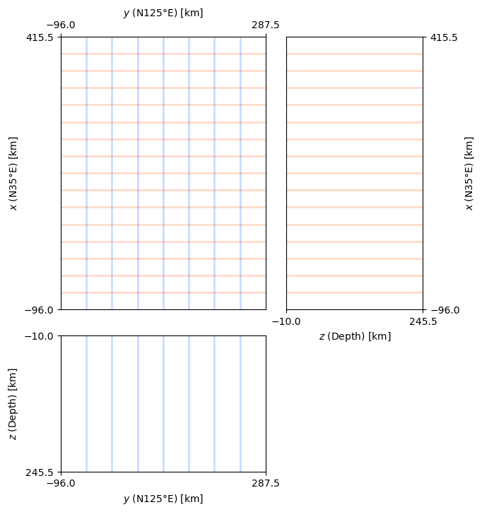
functions swpc.chkregion_2d() and swpc.chkregion_3d() enables us to confirm the model size and coordinate settings visually. Here is an example:

1
2
3
4
5
6
7
8
prm2 = swpc.prm_new()

prm2['nx'] = 1024
prm2['ny'] = 768
prm2['nz'] = 512
prm2['nproc_x'] = 16
prm2['nproc_y'] = 8
prm2['phi'] = 35
1
swpc.chkregion_2d(prm2);

1
swpc.chkregion_3d(prm2);

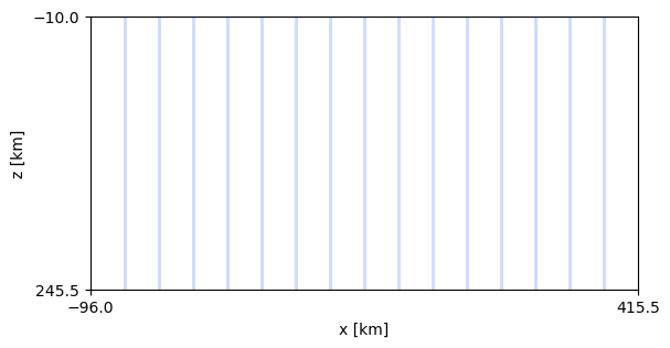
The model region is partitioned into MPI sub-regions by color lines.

Output waveforms

ObsPy is a de-facto standard on reading seismograms and applying basic manipulation of seismic data. Since the ObsPy can directly read the SAC-formatted seismogram, one can easily import the output waveform data generated by the OpenSWPC without any additional processings.

Note that some user reported that the ObsPy occasionaly fails to specify the format when it reads SAC files produced by OpenSWPC properly. It is recommended to add format='sac' option to obspy.read() function to explicitly tell this is SAC-formatted file.

1
ls /path/to/OpenSWPC/output/wav/swpc_N.N.AAKH.Vz.sac

/path/to/OpenSWPC/output/wav/swpc_N.N.AAKH.Vz.sac

1
import obspy
1
tr = obspy.read('/path/to/OpenSWPC/output/wav/*.Vz.sac', format='sac')
1
2
3
4
# set distance to stats
# original distance header in stats.sac.dist is not read by record section plot function in obspy
for t in tr:
    t.stats.distance = t.stats.sac.dist * 1000
1
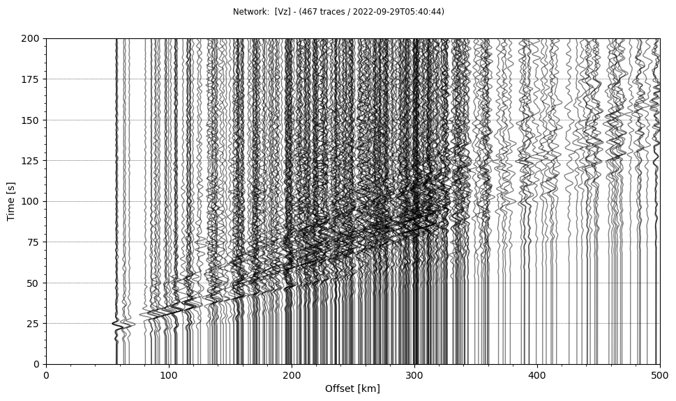
tr.plot(type='section', scale=5, offset_min=0, offset_max=500*1000, recordlength=200, reduce = 7).show()

png

1
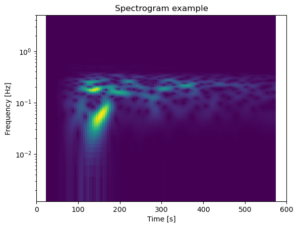
tr[10].spectrogram(wlen=60, log=True, title='Spectrogram example')

png

Output snapshots

2D snapshot data produced by OpenSWPC follows the CF metadata conventions of NetCDF format. There seems several libraries to read NetCDF files, and here is an exaple using xarray which has an affinity to the PyGMT.

1
fn_ob = '/path/to/OpenSWPC/output/swpc_N.ob.v.nc'
1
import xarray as xr
1
xr_ob = xr.open_dataset(fn_ob)

xarray dataset contains multiple list (array) data, as the NetCDF data format. Each data can be obtained by appending data varialbe name after . of the object:

1
xr_ob.topo.data
 1
 2
 3
 4
 5
 6
 7
 8
 9
10
11
12
13
array([[-3902.103 , -3902.103 , -3902.103 , ...,   841.1037,   841.1037,
          841.1037],
       [-3902.103 , -3902.103 , -3902.103 , ...,   841.1037,   841.1037,
          841.1037],
       [-3902.103 , -3902.103 , -3902.103 , ...,   841.1037,   841.1037,
          841.1037],
       ...,
       [-6059.085 , -6059.085 , -6059.085 , ..., -3449.3516, -3449.3516,
        -3449.3516],
       [-6059.085 , -6059.085 , -6059.085 , ..., -3449.3516, -3449.3516,
        -3449.3516],
       [-6059.085 , -6059.085 , -6059.085 , ..., -3449.3516, -3449.3516,
        -3449.3516]], dtype=float32)
1
xr_ob.lon.data
 1
 2
 3
 4
 5
 6
 7
 8
 9
10
11
12
13
array([[137.7886 , 137.788  , 137.78738, ..., 136.83992, 136.83867,
        136.8374 ],
       [137.80438, 137.80377, 137.80316, ..., 136.85922, 136.85797,
        136.85672],
       [137.82018, 137.81956, 137.81895, ..., 136.87854, 136.87729,
        136.87604],
       ...,
       [146.17456, 146.17517, 146.17578, ..., 147.11504, 147.11627,
        147.11752],
       [146.19035, 146.19096, 146.19157, ..., 147.13434, 147.13559,
        147.13684],
       [146.20613, 146.20674, 146.20737, ..., 147.15364, 147.1549 ,
        147.15616]], dtype=float32)
1
xr_ob.lat.data
 1
 2
 3
 4
 5
 6
 7
 8
 9
10
11
12
13
array([[31.725807, 31.7393  , 31.752792, ..., 46.056538, 46.06998 ,
        46.08342 ],
       [31.72633 , 31.739822, 31.753315, ..., 46.05741 , 46.070854,
        46.084293],
       [31.726849, 31.740343, 31.753836, ..., 46.05828 , 46.07172 ,
        46.085163],
       ...,
       [31.727022, 31.740515, 31.754007, ..., 46.058567, 46.07201 ,
        46.085453],
       [31.726503, 31.739996, 31.753489, ..., 46.0577  , 46.071144,
        46.084583],
       [31.725983, 31.739475, 31.752968, ..., 46.056828, 46.07027 ,
        46.083714]], dtype=float32)

... and time slice of the wavefield can be reffered by the sequential time step number like

1
xr_ob.Vz[50].data
1
2
3
4
5
6
7
array([[0., 0., 0., ..., 0., 0., 0.],
       [0., 0., 0., ..., 0., 0., 0.],
       [0., 0., 0., ..., 0., 0., 0.],
       ...,
       [0., 0., 0., ..., 0., 0., 0.],
       [0., 0., 0., ..., 0., 0., 0.],
       [0., 0., 0., ..., 0., 0., 0.]], dtype=float32)

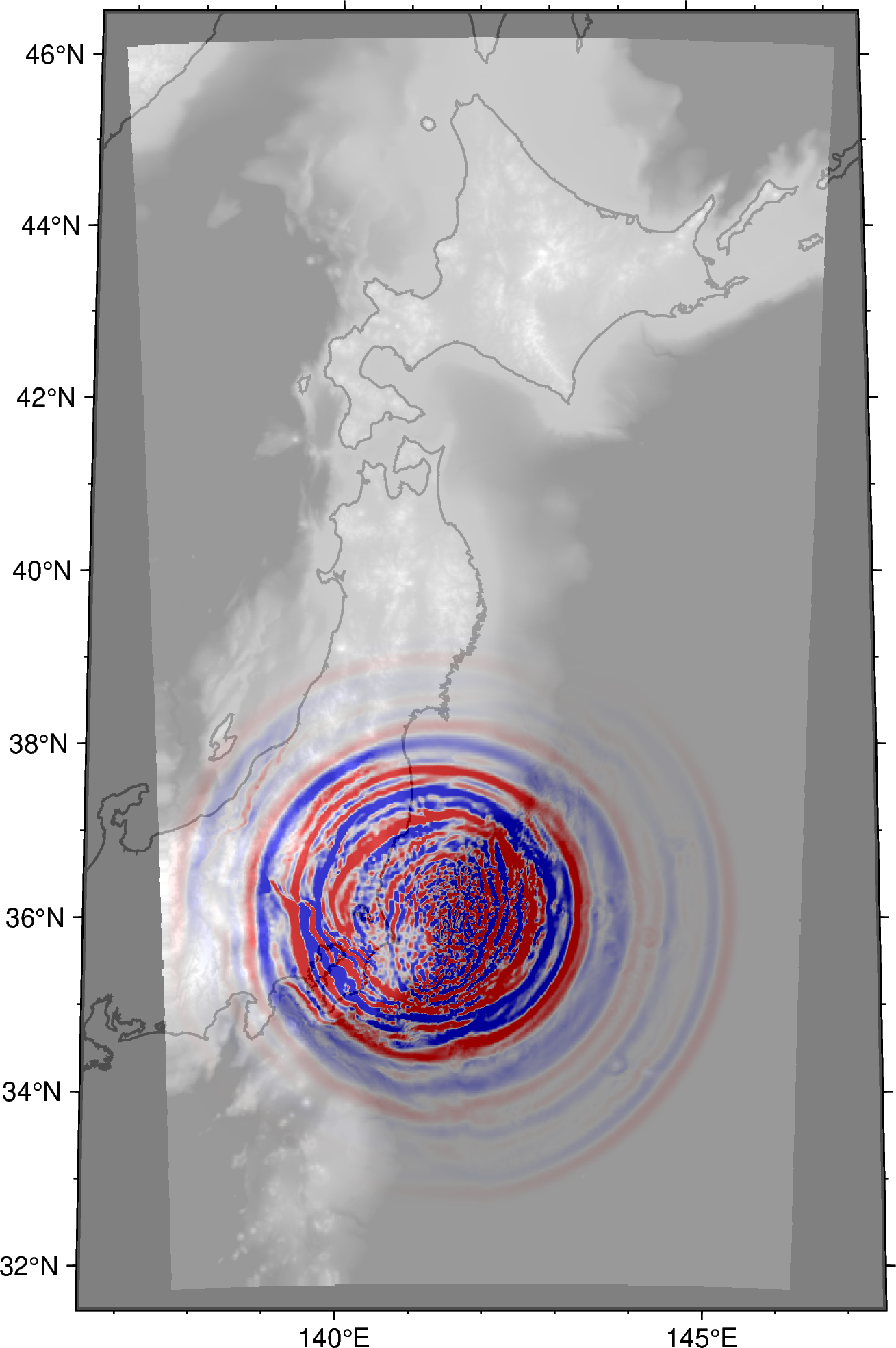
Note that the OpenSWPC performs simulations in the Cartesian coordinate. The result is mapped to the geographical cooridnate upon output, but the data is not evenly-spaced in longitude-latitude system. Thus, interpolation and/or resampling may be necessary to plot the wavefield on a map.

1
2
import pygmt
import numpy as np
 1
 2
 3
 4
 5
 6
 7
 8
 9
10
11
12
13
14
15
16
17
# make interpolated grid data by nearneighbor function

region = [136.5, 147.5, 31.5, 46.5]
spacing = 0.01
radius = 0.05

# topography grid
grd_topo = pygmt.nearneighbor(x = xr_ob.lon.data.ravel(), 
                              y = xr_ob.lat.data.ravel(),
                              z = xr_ob.topo.data.ravel(), 
                              region = region, spacing = spacing, search_radius = radius) 

# wavefield at 50th time step
grd_wave = pygmt.nearneighbor(x = xr_ob.lon.data.ravel(), 
                              y = xr_ob.lat.data.ravel(),
                              z = xr_ob.Vz[50].data.ravel(), 
                              region = region, spacing = spacing, search_radius = radius) 
 1
 2
 3
 4
 5
 6
 7
 8
 9
10
11
12
13
14
15
16
fig = pygmt.Figure()

with pygmt.config(MAP_FRAME_TYPE  = 'plain'):

    # background topography
    pygmt.makecpt(cmap='gray', series=[-2000, 2000, 500], continuous=True)
    fig.grdimage(grid=grd_topo, projection='N142/10c', region=region, frame=['WSen', 'xaf', 'yaf'])

    # coastline
    fig.coast(resolution = 'h', area_thresh = 100, shorelines='thin,black')

    # wavefield with tranparency
    pygmt.makecpt(cmap='polar',series = [-0.1, 0.1, 0.02], continuous=True, background=True)
    fig.grdimage(grid=grd_wave, transparency=40)

fig.show()

png