New features¶

Version 26.09.1 (2026-09-13)¶

This is a minor bug-fix version.

Fix the improper calculation of epicentral distance and event location in SAC headers in single-force mode
Improved horizontal boundary treatment for PML, which is particularly efficient to reduce artificial reflection in plane-wave mode

Version 26.09 (2026-09-01)¶

Viscoelastic PML¶

In previous versions of OpenSWPC, the medium within the Perfectly Matched Layer (PML) region was assumed to be perfectly elastic (Maeda et al., 2017). Although this assumption simplified the computation, particularly in strongly attenuating media it failed to reproduce the frequency-independent velocity reduction associated with physical dispersion. The resulting velocity mismatch between the interior and PML regions could generate artificial reflected waves.

Starting with this version, the PML has been combined with exactly the same Generalized Zener Body viscoelastic model as that used in the interior region (Martin and Komatitsch (2009)), substantially improving the performance of the PML.

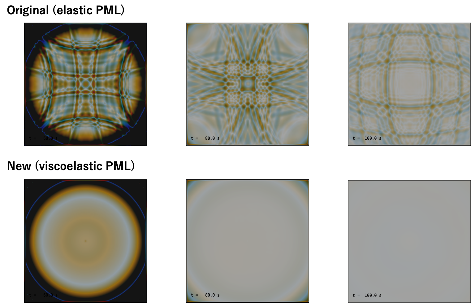
Viscoelastic PML — Snapshots of seismic-wave velocity amplitudes at the surface in a homogeneous medium with intrinsic attenuation of $Q_P = Q_S = 30$ . The upper panel shows the previous implementation, and the lower panel shows the new implementation. Small amplitudes relative to the direct waves are enhanced for visualization.

The above figure compares the performance of the previous and new absorbing boundary conditions. The previous method produced weak artificial reflected waves, whereas these reflections are drastically reduced with the new viscoelastic PML. This improvement is also expected to enhance the stability of the PML.

Although the new algorithm itself increases both computational cost and memory requirements, the memory-saving improvements described below, together with the associated performance gains, result in lower overall memory usage than in previous versions in most cases. Depending on the computing environment, the computation time ranges from approximately the same as before to an increase of at most about 15%.

Reduction of memory usage¶

Memory usage has been significantly reduced by redesigning the allocation of array variables required only within the PML regions and by carefully reassessing which variables actually require FP64 (double-precision) arithmetic in the mixed-precision implementation using FP64 and FP32 (single precision).

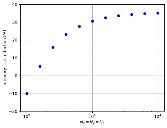
Memory reduction — Reduction in required memory in the new version relative to the previous version for models with equal numbers of grid points along all three dimensions ( $N_x = N_y = N_z$ ).

The above figure shows the reduction in required memory in Version 26.09 relative to Version 25.05, including the effects of the new PML implementation described above. For small models, the increase in memory usage associated with the viscoelastic PML has a relatively large impact. As the model size increases, however, the benefits of the memory reductions become more pronounced. For grid dimensions commonly used in three-dimensional seismic-wave propagation simulations ( $10^3 \sim 10^4$ ), memory usage is reduced by more than 30%.

Color Universal Design (CUD) for `read_snp.x`¶

The visualization of snapshot files by the bundled read_snp.x tool previously used reddish and greenish colors for the two types of data. In Version 26.09, a new color palette designed to accommodate diverse color vision has been introduced and is available through the -color cud option. A new -bgsat option has also been added to adjust the saturation of the background colors representing topography and velocity structure.

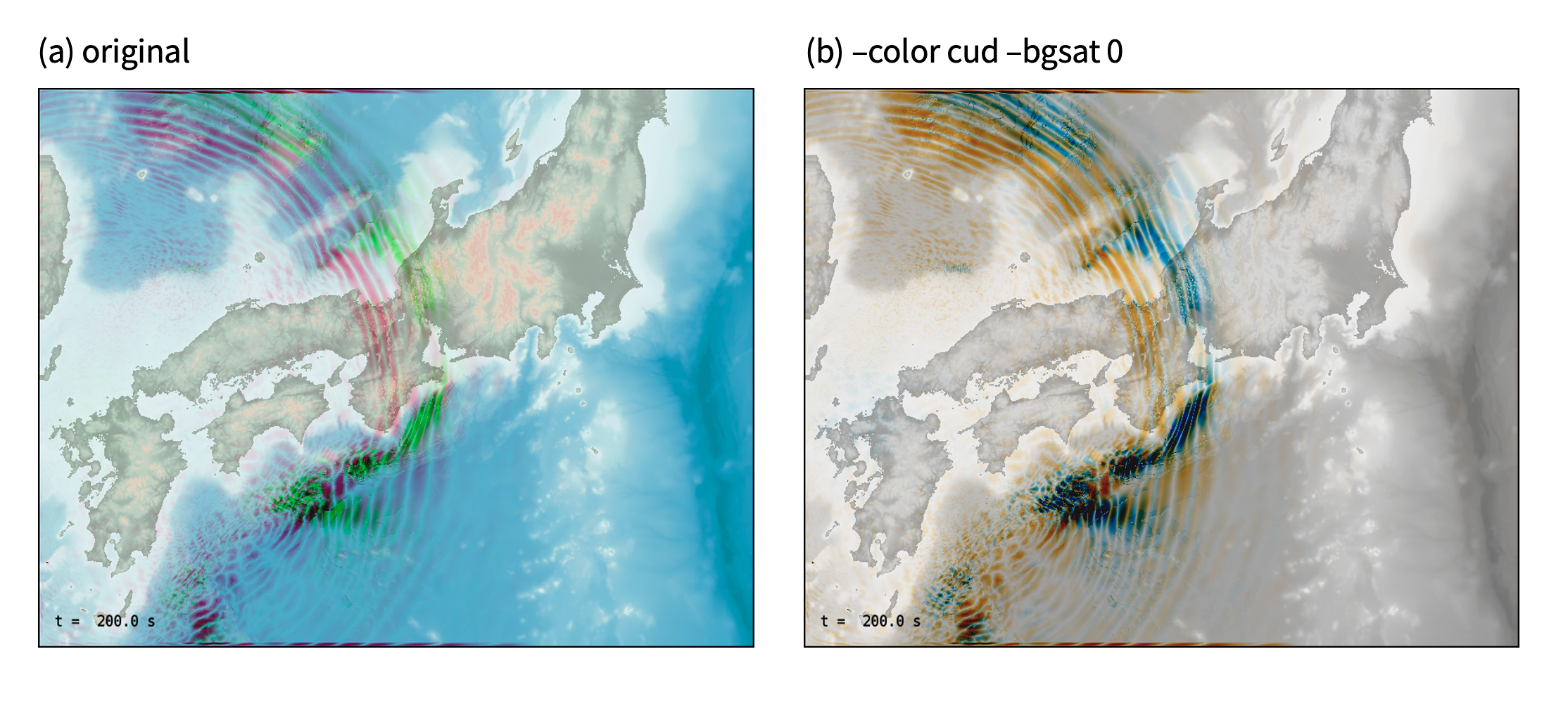
Comparison of color modes for visualization with `read_snp.x`.

Fullspace mode reactivated¶

The fullspace_mode, which places a PML also at the upper boundary of the model where an absorbing boundary condition is normally unnecessary because of the vacuum (air) layer, has been reintroduced.

This mode was implemented between Versions 5.0 and 5.1, but was subsequently withdrawn because of technical problems encountered at the time. Since the PML implementation has been rewritten in Version 26.09, those earlier problems no longer apply.

A new source time function¶

Asymmetric cosine function asymcos (Ji et al., 2003) is implemented as a new source time function.

Updated preset build environments¶

makefile.arch and makefile-tools.arch have been reorganized, and two examples for GPU-based systems have been added.

Removed features¶

Waveform: csf-format¶

Waveform format 'csf' was removed. Alternatively, please consider using tar_st or tar_node format files.

Snapshot: native-format¶

As of this version, only NetCDF-formatted snapshot data is spported.

Removal of the `csf` waveform format¶

Support for waveform output in the proprietary csf format has been removed. To combine multiple waveform files into a single output file, the tar_st or tar_node formats can now be used. These formats store SAC files in a tar archive.

Version-dependent manual¶

The appropriate manual for each OpenSWPC version can now be selected using the version selector at the top of the manual website. Manuals for Version 25.05 and earlier are provided collectively as legacy.

Version 25.05 (2025-05-20)¶

GPGPU-Ready¶

This is the first version to support GPGPU computing via OpenACC.

All simulation codes (swpc_3d, swpc_psv swpc_sh) now support many-GPU computing using OpenACC and MPI, enabling ultra-high-speed operation.
Supporting tools can also be compiled with NVIDIA's nvfortran and run properly not only on x86 architectures but also on NVIDIA Grace CPUs.

Version 25.01 (2025-01-04)¶

Velocity Structure Model Linear Gradient Model (`lgm`)¶

It is now possible to create a model in which seismic wave velocity varies linearly within a layer, using the same format input file as the Lateral Homogeneous Medium (lhm). This allows the user to apply a velocity structure that smoothly changes with depth to simulations.

The figures below show PS snapshots of the P-SV code for vmodel=“lhm” and vmodel=“lgm” using the same structural model file provided in the OpenSWPC example. Compared to lhm, lgm has a relatively simple wave field, with fewer reflected and converted waves at the internal boundary due to the absence of the velocity discontinuity surface (the gray horizontal line).

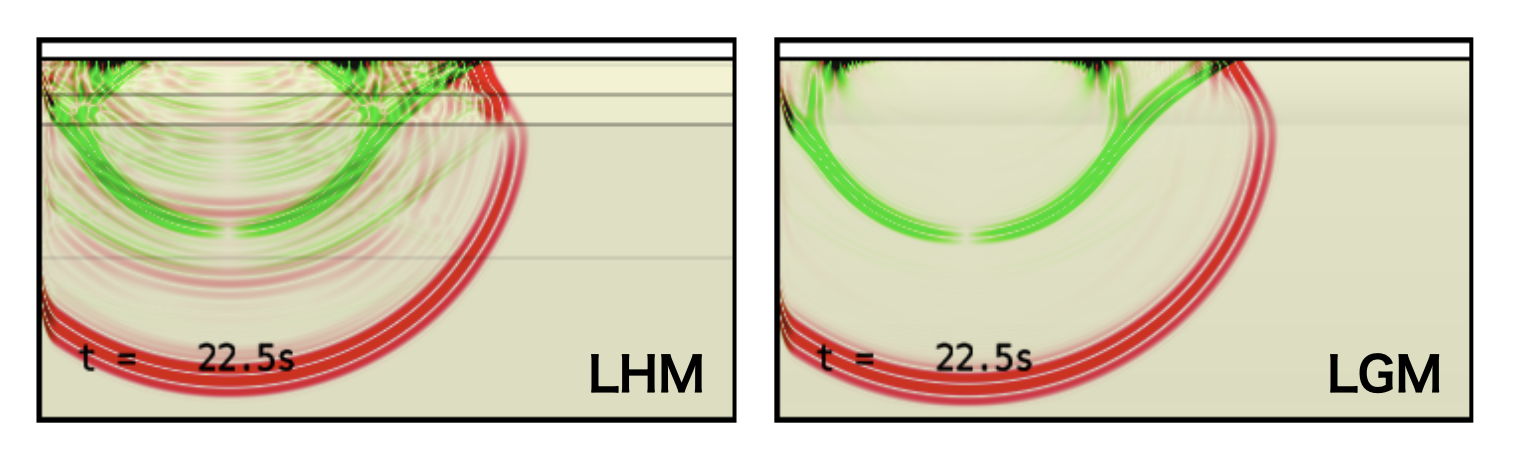
Example of a numerical simulation snapshot of `swpc_psv` using the structural model file `example/lhm.dat`. The left image was calculated using `vmodel=“lhm”` and the right image was calculated using `vmodel=“lgm”`.

On the other hand, the lgm model can also express velocity discontinuity surfaces. In other words, lgm is a superset that includes lhm. In addition, lgm_rmed, which corresponds to lhm_rmed with a random medium superimposed, is also provided.

`tar` archive format for waveform output¶

A function has been added to output seismic waveform files in SAC format as a single tar archive for each observation point or for all waveforms from the output node (wav_format = “tar_st”, wav_format = “tar_node”).

Since tar is an archive for a single file and does not include compression, the size of the output file will not change much. However, by reducing the number of output files through archiving, it is expected that data output will be more efficient and that file management after output will be easier.

If one use the seismology library ObsPy in Python, one can read the SAC waveform files that have been archived as tar without extracting them.

Until now, the proprietary binary csf format has been provided as a format for combining multiple waveform data into a single file. As the purpose of this format is duplicated, csf output is depreciated and will be removed in future versions.

Epicentral distance in waverform files¶

The default behavior is now to record the epicentral distance in the header of the waveform file, which was previously an optional function controlled by the calc_wav_dist parameter. The calc_wav_dist parameter has been removed.

Change in output file name¶

The problem of overwriting output file names due to duplication when executing the SH, P-SV and 3D codes from the same input parameter file has been resolved. For this reason, the code name is now added to the output file name.

In addition, images and data output from read_snp.x are now divided into directories by type.

Documentation update¶

The entire documentation was reviewed; outdated information was updated, as well as the explanations were reinforced.

Minor bugfixes¶

Fixed a problem where the waveform time could not be read correctly in some environments due to the SAC header nzmsec being undefined
Fixed a problem where the initial value -12345 of the SAC header kf was not output correctly
Corrected the UT-LocalTime discrepancy in the time stamps recorded in the waveform and snapshot output
Fixed the file name in the JIVSM structure model creation script
Addressed the issue of the output directory sometimes failing to be created on a shared file system

Version 24.09 (2024-09-13)¶

Starting with this release, OpenSWPC uses the Calender Versioning scheme. The version number is determined by YY.0M (year and month with zero padding).

High-speed snapshot data export¶

By using a new algorithm, snapshot data export is significantly accelerated, resulting in a maximum reduction of ~20% of the total computation time for 3D simulation.

Waveform output during calculation¶

Previously, seismic waveform files were not created at a station until all calculations were completed. By setting the new parameter ntdec_wav_prg, waveforms are periodically output during the computation. The waveform amplitudes for the parts of the waveform that have not yet been computed are filled with zeros. This new feature allows users to monitor the computation in the middle of a calculation. However, be careful not to use too frequent output, as it may affect the speed of the computation.

Remove Checkpointing/Restarting functionality¶

In order to continue to improve the code, we have decided to remove the Checkpointing/Restarting feature, which we believe is now rarely used. If you wish to use this feature, we recommend that you continue to use Version 5.3.1. There is no difference in calculation results between this version and Version 5.3.1.

NetCDF is always needed¶

Until now, it was not impossible to compile without the NetCDF library. However, since it is impractical to use this tool without NetCDF, we have simplified the code by always requiring a link to the NetCDF library at compile time.

Code modernization¶

We have eliminated the old Fortran90/95 era syntax and #ifdef-#endif macro branches that were maintained for compatibility with some past supercomputers, and rewritten much of the code in the simpler and more modern notation of Fortran2003 and later. Some newer Fortran 2008 syntax is included, but we are pretty confident that it is within the scope of most compilers currently available.

Version 5.3.1 (2024-04-14)¶

Version information option¶

All executables (binaries with a .x filename extension in the bin/ directory) now accept -v or --version options to display the current version number, as shown below.

% ./bin/swpc_psv.x -v
swpc_psv (OpenSWPC) version 5.3.1

Repository change¶

Starting with version 5.3.1, code will be released from the new organizational repository (https://github.com/OpenSWPC/OpenSWPC). Links to the old repository will be redirected to the new one, and the old version of the information will not be lost. Also, starting with this release, the online documentation will be maintained separately from the OpenSWPC source code. The documentation repository is https://github.com/OpenSWPC/OpenSWPC.github.io.

A new organization repository (https://github.com/OpenSWPC/OpenSWPC)

Version 5.3.0 (2023-02-02)¶

Better parallel partitioning¶

In previous versions, automatic MPI area allocation sometimes failed when the number of grids in the X or Y direction was not divisible by the number of MPI partitions and the number of MPI partitions was very large.

This problem has been fixed in version 5.3.0.

In new version, the partitioning algorithm is as follows:

Let $N$ be the number of grid, and $P$ the number of MPI partitions. If $N$ is divisible by $P$ , i.e., $\mod(N,P)= 0$ , the number of grids assigned to a node is $N_P = N/P$ . If this is not the case, the following rule is applied:

Node ID	Number of Grids $N_P$
0 to $P$ - $M$ -1	$N_P = (N-M)/P$
$P$ - $M$ to $P$ -1	$N_P = (N-M)/P + 1$

(where $M = \mod(N,P)$ )

Python integration¶

An example of processing OpenSWPC input/output in Python is included in this manual.

Updated documentation¶

Try OpenSWPC on cloud¶

See this example. This is also would be a nice guide to compile the OpenSWPC in Ubuntu Linux.

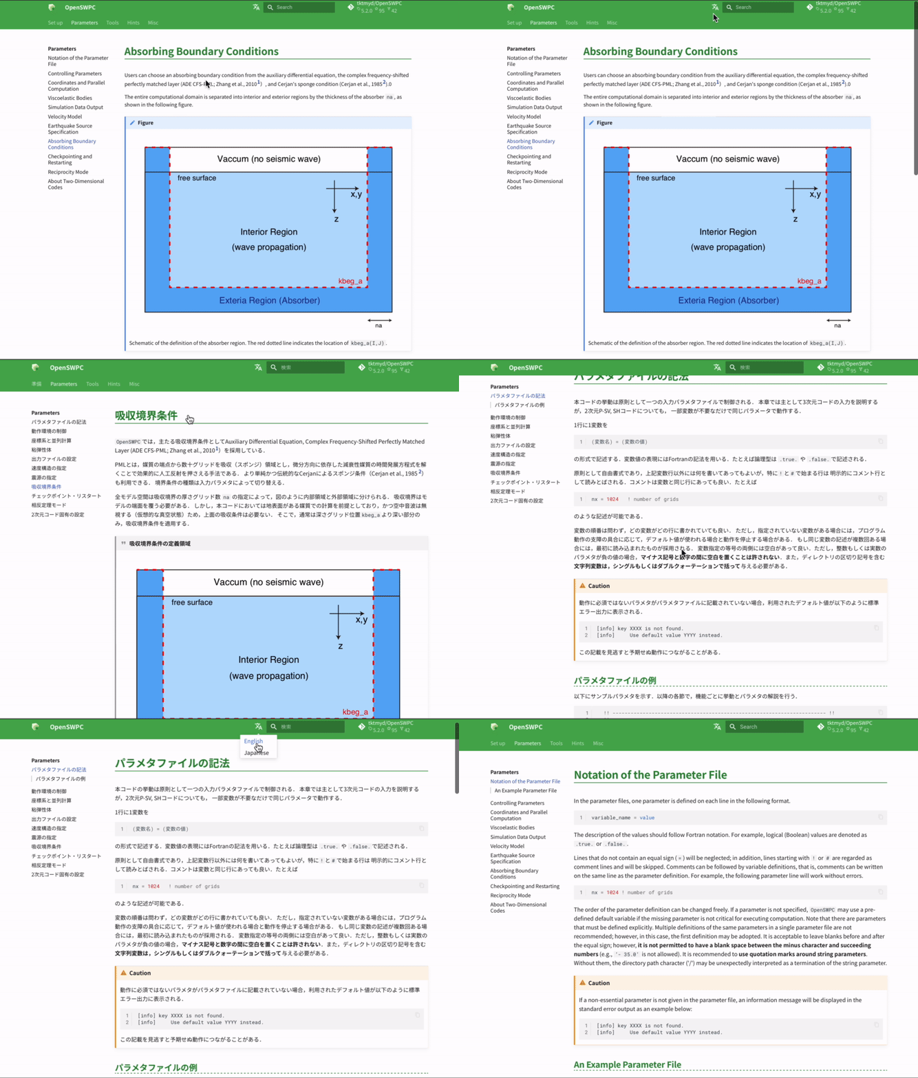
Better switching between EN/JP documentation¶

One can switch between Japanese and English documentation using the button to the left of the search box.
Untranslated documents (for example, this page) are displayed in English even in Japanese mode.

Others¶

Tune-up in some supercomputers
Updated version of Japanese community model JIVSM.

Previous Revision Histories¶

2021-08-27 (v5.2.0): Earth-flattening transformation, psmeca (a new source representation), seawater velocity structure w/ SOFAR channel, a new tool that converts 2D simulation output into pseudo-3D, supporting new Japanese supercomputers, and some minor bugfixes.
2020-08-13 (v5.1.0): Strict-mode
2019-08-27 (v5.0.0): New web-based documentation, stress/strain waveform output, slip-based source specification, and many bugfixes.
2017-09-21 (v4.0): Minor bugfixes, new binary output for waveform, updated references.
2016-08-20 (v3.0): Hybrid parallel simulation for 2D codes.
2016-06-19 (v2.0): Hybrid parallel simulation for 2D codes.
2016-05-05 (v1.0): Official first release as an open-source software
2016-02-03: Output in \texttt{NetCDF} format.
2016-01-14: Body force and reciprocity modes.
2015-07-14: MPI/OpenMP hybrid parallel simulation mode.
2015-06-29: Added random media.
2015-06-10: Revision for the new Earth Simulator.
2015-06-04: First closed version for the ERI/UT joint usage program.